Python OpenCV Filters Test

26 Sep 2019 in Devlog / MLDLStudy on Ml, Python-opencv

애니메이션 캐릭터 얼굴의 엣지를 찾기 위해 다양한 엣지 검출 알고리즘으로 테스트를 수행해본 결과를 공유합니다.

본 글은 애니메이션 캐릭터 얼굴의 엣지를 찾기 위해 다양한 엣지 검출 알고리즘으로 테스트를 수행해본 결과입니다.

ConvertLineDrawing using conv and maxpool in Pytorch

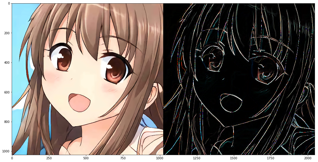
먼저 Qiita의 koshian2가 제안하는 방법을 사용해 엣지를 검출해 보겠습니다. 전체 코드는 여기서 확인하실 수 있고, 유저 wakame1367가 해당 소스 코드를 캐글 커널로 만들어 공개했습니다. 각 링크에서 더 자세한 정보를 확인하실 수 있습니다.

import numpy as np
from PIL import Image
import torch
import torch.nn.functional as F
import matplotlib.pyplot as plt
from torchvision.utils import make_grid

def load_tensor(image_path):
    with Image.open(image_path) as img:
        array = np.asarray(img, np.float32) / 255.0 # [0, 1]
        array = np.expand_dims(array, axis=0)
        array = np.transpose(array, [0, 3, 1, 2]) # pytorch 채널 순서인 NCHW 순서로 transpose
        return torch.as_tensor(array)

def show_tensor(input_image_tensor):
    img = input_image_tensor.numpy() * 255.0
    img = img.astype(np.uint8)[0,0,:,:]    
    plt.imshow(img, cmap="gray")
    plt.show()

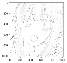
def linedraw(image_path):
    # 데이터 로드
    x = load_tensor(image_path)
    # Y = 0.299R + 0.587G + 0.114B를 이용해 Grayscale로 변경
    gray_kernel = torch.as_tensor(
        np.array([0.299, 0.587, 0.114], np.float32).reshape(1, 3, 1, 1))
    x = F.conv2d(x, gray_kernel) 
    dilated = F.max_pool2d(x, kernel_size=3, stride=1, padding=1)
    diff = torch.abs(x-dilated)
    # 반전
    x = 1.0 - diff
    # 결과 보기
    show_tensor(x)

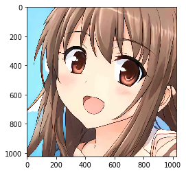
테스트를 위한 이미지를 로드합니다. 경로는 여러분의 환경에 맞도록 바꿔 주세요.

from pathlib import Path
image_path = Path('ExampleImgs/example-1006.jpg')
img = linedraw(image_path)
img

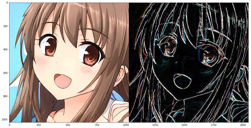
이어서, 엣지 검출을 ①Hard-coded kernel과 ②OpenCV 제공 함수를 이용해 진행해 보겠습니다. 우선 테스트를 위한 이미지를 다시 로드하겠습니다. 아래 테스트는 ‘파이썬으로 만드는 OpenCV 프로젝트’책과 위키피디아를 참고해 진행했습니다.

import cv2
import numpy as np
import matplotlib.pyplot as plt

img_path = 'ExampleImgs/example-1006.jpg'
img = cv2.imread(img_path)
img = cv2.cvtColor(img, cv2.COLOR_BGR2RGB)

plt.imshow(img)

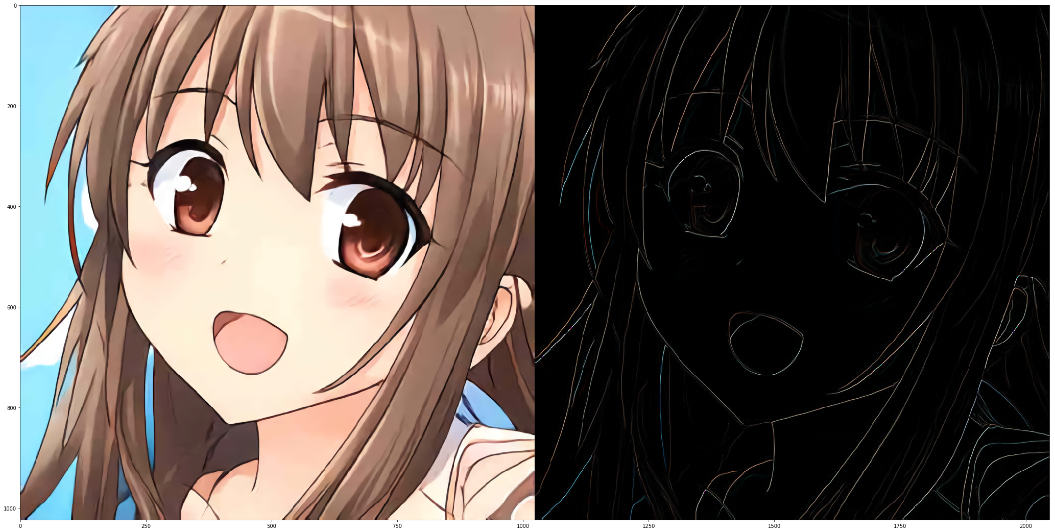
Basic Gradient Kernel

가장 기본적인 엣지 검출 알고리즘입니다. 엣지 검출을 위해서는 이미지의 픽셀값 변화가 갑자기 커지는 부분을 찾아내야 하며, 연속된 픽셀값에 미분을 수행하면 이 변화량을 구할 수 있습니다. 가장 기본적인 미분은 영상 속 픽셀 데이터를 이산화한 후 X축과 Y축 각각의 방향을 기준으로 다음 픽셀에서 현재 픽셀의 값을 빼는 것입니다.
아래 코드는 X방향과 Y방향 각각에 대한 미분 마스크를 생성한 후 cv2.filter2D로 넘겨 합성곱 연산(Convolution)을 수행합니다. X방향 미분 마스크는 세로 방향에 대한 엣지를 검출하고, Y방향 미분 마스크의 합성곱 결과는 가로 방향의 엣지를 검출합니다. discrete한 근사값으로 얻어낸 미분 결과물이지만 이를 기울기(Gradient)라고 부릅니다.

결과로 나온 edge_gx와 edge_gy를 더해 최종 결과물을 얻어 봅시다.

plt.figure(figsize=(60, 20))
left = 0.125
right = 0.7
bottom = 0.2
top = 0.9
wspace = 0.02
hspace = 0.0
plt.subplots_adjust(left=left, right=right, bottom=bottom, top=top, wspace=wspace, hspace=hspace)

# Create gradient kernel
gx_kernel = np.array([[-1,1]])
gy_kernel = np.array([[-1],[1]])

# Apply filter to image
edge_gx = cv2.filter2D(img, -1, gx_kernel)
edge_gy = cv2.filter2D(img, -1, gy_kernel)

# Print results
merged = np.hstack((img, edge_gx+edge_gy))
plt.imshow(merged)

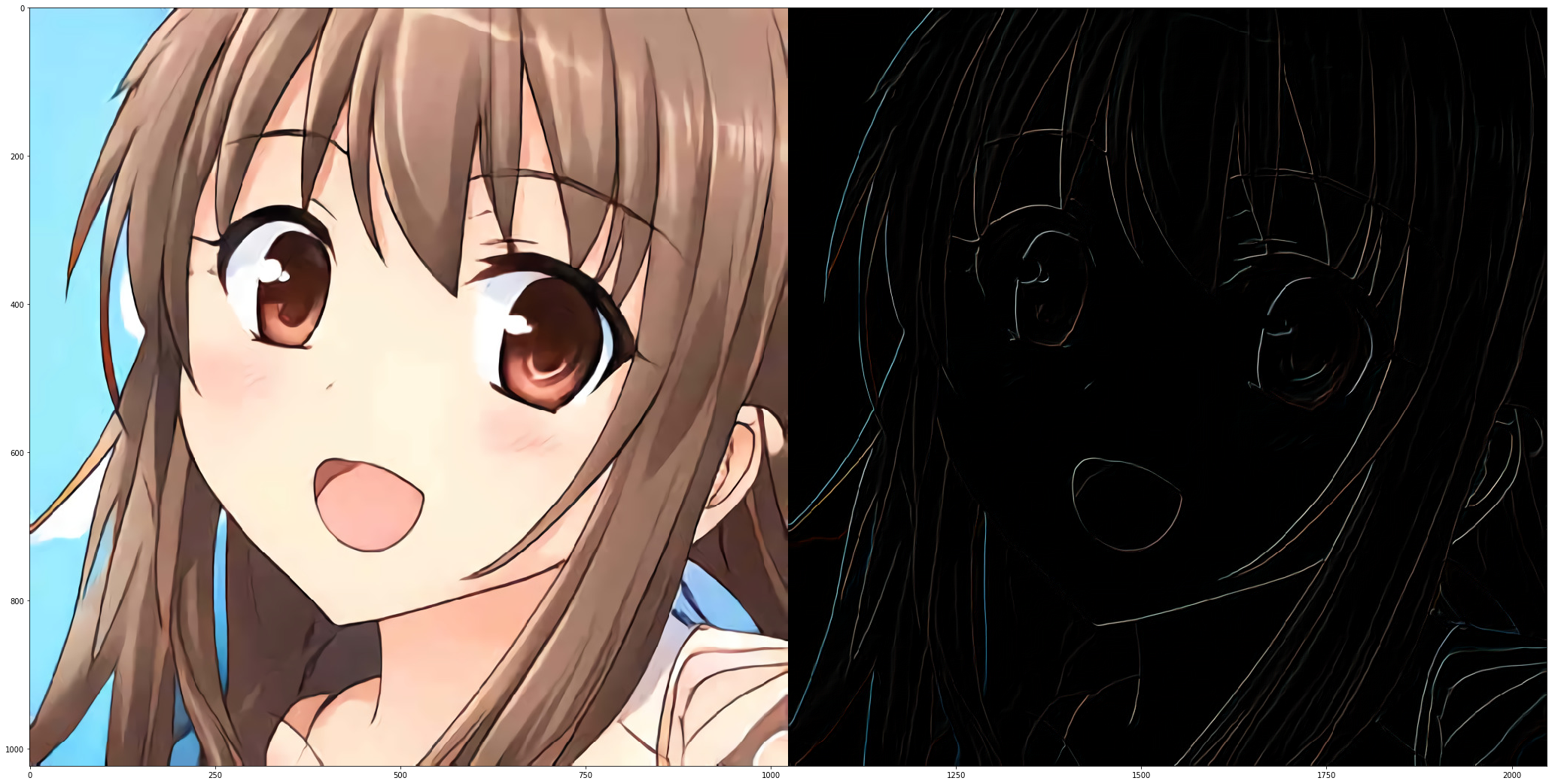
Roberts Mask

1963년 로렌스 로버츠(Lawrence Roberts)가 기본 미분 커널을 개선해 제안한 커널로, 사선 경계 검출 효과를 높였으나 노이즈에 민감하고 엣지 강도가 약한 단점이 존재합니다. 기본 미분과 비슷하게 두 축에 대해 합성곱 연산을 수행한 결과물을 더해 최종 결과물을 얻어 봅시다.

plt.figure(figsize=(60, 20))
left = 0.125
right = 0.7
bottom = 0.2
top = 0.9
wspace = 0.02
hspace = 0.0
plt.subplots_adjust(left=left, right=right, bottom=bottom, top=top, wspace=wspace, hspace=hspace)

# Create Roberts kernel
gx_kernel = np.array([[1,0],[0,-1]])
gy_kernel = np.array([[0,-1],[-1,0]])

# Apply kernel to image
edge_gx = cv2.filter2D(img, -1, gx_kernel)
edge_gy = cv2.filter2D(img, -1, gy_kernel)

# Print results
merged = np.hstack((img, edge_gx+edge_gy))
plt.imshow(merged)

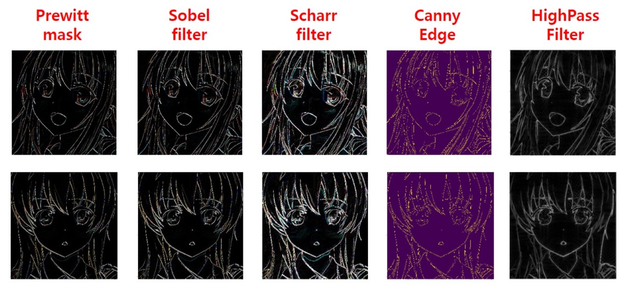
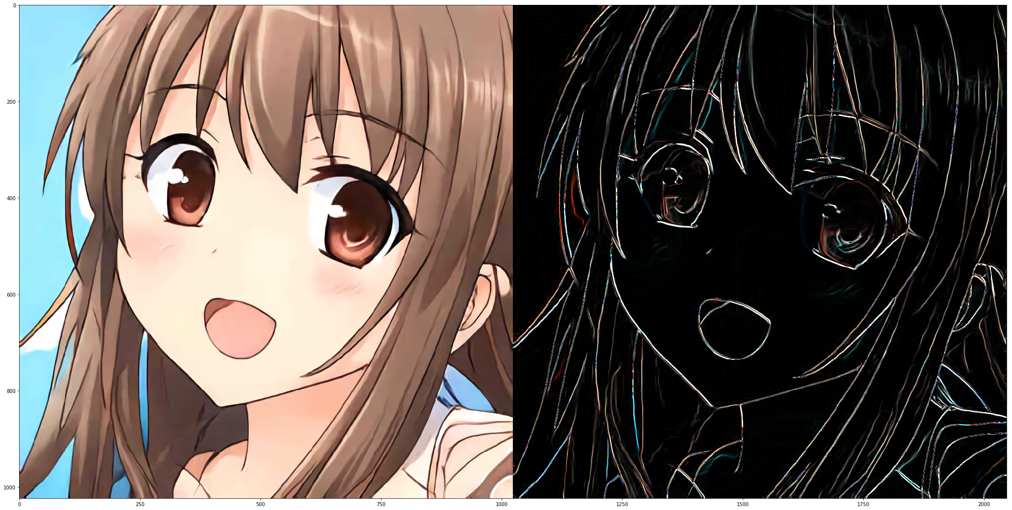
Prewitt mask

프리윗 마스크는 주디스 프리윗(Judith M. S. Prewitt)이 제안한 마스크로, 각 방향에 대해 차분을 세 번 계산하도록 배치했기 때문에 엣지 강도가 강하게 검출되며, 수직 및 수평 엣지를 동등하게 찾는 장점이 있으나 대각선 검출에 취약한 마스크입니다.

plt.figure(figsize=(60, 20))
left = 0.125
right = 0.7
bottom = 0.2
top = 0.9
wspace = 0.02
hspace = 0.0
plt.subplots_adjust(left=left, right=right, bottom=bottom, top=top, wspace=wspace, hspace=hspace)

# Create Prewitt kernel
gx_kernel = np.array([[-1,0,1],[-1,0,1],[-1,0,1]])
gy_kernel = np.array([[-1,-1,-1],[0,0,0],[1,1,1]])

# Apply kernel to image
edge_gx = cv2.filter2D(img, -1, gx_kernel)
edge_gy = cv2.filter2D(img, -1, gy_kernel)

# Print results
merged = np.hstack((img, edge_gx+edge_gy))
plt.imshow(merged)

Sobel filter

유명한 필터 중 하나인 소벨 필터는 1968년 어원 소벨(Irwin Sobel)이 제안한 필터로, 중심 픽셀의 차분 비중을 두 배로 주어 수평 및 수직 대각선 경계 검출에 모두 강한 마스크입니다. 가장 대표적인 1차 미분 마스크로써, 전용 함수를 OpenCV에서 제공해 줍니다.

• dst = sv2.Sobel(src, ddepth,dx, dy[, dst, ksize, scale, delta, borderType])
  • src : 입력 이미지(Numpy array)
  • ddepth : 출력 영상의 dtype (-1 : 입력 영상과 동일한 타입)
  • dx, dy : 미분 차수 (0, 1, 2중 선택 가능하며, 둘 다 0일수는 없음.)
  • ksize : 커널의 사이즈 (1, 3, 5, 7중 선택 가능)
  • scale : 미분에 사용할 계수
  • delta : 연산 결과에 더할 가중치

하지만 소벨 필터는 커널의 크기가 작은 경우 또는 커널의 크기가 크더라도 그 중심에서 멀어질수록 엣지 방향의 정확도가 떨어지는 단점이 존재합니다.

plt.figure(figsize=(60, 20))
left = 0.125
right = 0.7
bottom = 0.2
top = 0.9
wspace = 0.02
hspace = 0.0
plt.subplots_adjust(left=left, right=right, bottom=bottom, top=top, wspace=wspace, hspace=hspace)

# Create Sobel kernel
gx_kernel = np.array([[-1,0,1],[-2,0,2],[-1,0,1]])
gy_kernel = np.array([[-1,-2,-1],[0,0,0],[1,2,1]])

# Apply kernel to image
edge_gx = cv2.filter2D(img, -1, gx_kernel)
edge_gy = cv2.filter2D(img, -1, gy_kernel)

# Using Sobel API in OpenCV
sobelx = cv2.Sobel(img, -1, 1, 0, ksize=3)
sobely = cv2.Sobel(img, -1, 0, 1, ksize=3)

# Print results
merged_hardcoded = np.hstack((img, edge_gx+edge_gy))
merged_sobel = np.hstack((img, sobelx+sobely))
# plt.subplot(211)
# plt.imshow(merged_hardcoded)
plt.subplot(212)
plt.imshow(merged_sobel)

Scharr filter

샤르 필터는 위에서 언급한 소벨 필터의 단점을 개선한 필터입니다.

dst = sv2.Scharr(src, ddepth,dx, dy[, dst, scale, delta, borderType])

plt.figure(figsize=(60, 20))
left = 0.125
right = 0.7
bottom = 0.2
top = 0.9
wspace = 0.02
hspace = 0.0
plt.subplots_adjust(left=left, right=right, bottom=bottom, top=top, wspace=wspace, hspace=hspace)

# Create Sobel kernel
gx_kernel = np.array([[-3,0,3],[-10,0,10],[-3,0,3]])
gy_kernel = np.array([[-3,-10,-3],[0,0,0],[3,10,3]])

# Apply kernel to image
edge_gx = cv2.filter2D(img, -1, gx_kernel)
edge_gy = cv2.filter2D(img, -1, gy_kernel)

# Using Scharr API in OpenCV
scharrx = cv2.Scharr(img, -1, 1, 0)
scharry = cv2.Scharr(img, -1, 0, 1)

# Print results
# merged_hardcoded = np.hstack((img, edge_gx+edge_gy))
merged_scharr = np.hstack((img, scharrx+scharry))
# plt.subplot(211)
# plt.imshow(merged_hardcoded)
plt.subplot(212)
plt.imshow(merged_scharr)

Laplacian filter

1차 미분 결과에 대해 다시 한번 미분을 수행하면(2차 미분) 경계를 좀 더 확실히 검출할 수 있습니다. 라플라시안 필터는 대표적인 2차 미분 필터 중 하나로, OpenCV에서는 소벨 필터와 마찬가지로 cv2.Laplacian()함수를 제공하고 있습니다.

dst = sv2.Laplacian(src, ddepth[, dst, ksize, scale, delta, borderType])

라플라시안 필터는 노이즈에 민감하기 때문에 가우시안 블러 필터로 어느 정도 노이즈를 경감시키고 적용하는 것이 좋습니다.

plt.figure(figsize=(60, 20))
left = 0.125
right = 0.7
bottom = 0.2
top = 0.9
wspace = 0.02
hspace = 0.0
plt.subplots_adjust(left=left, right=right, bottom=bottom, top=top, wspace=wspace, hspace=hspace)

# Using Laplacian API in OpenCV
edge = cv2.Laplacian(img, -1)

# Print results
merged = np.hstack((img, edge))
plt.imshow(merged)

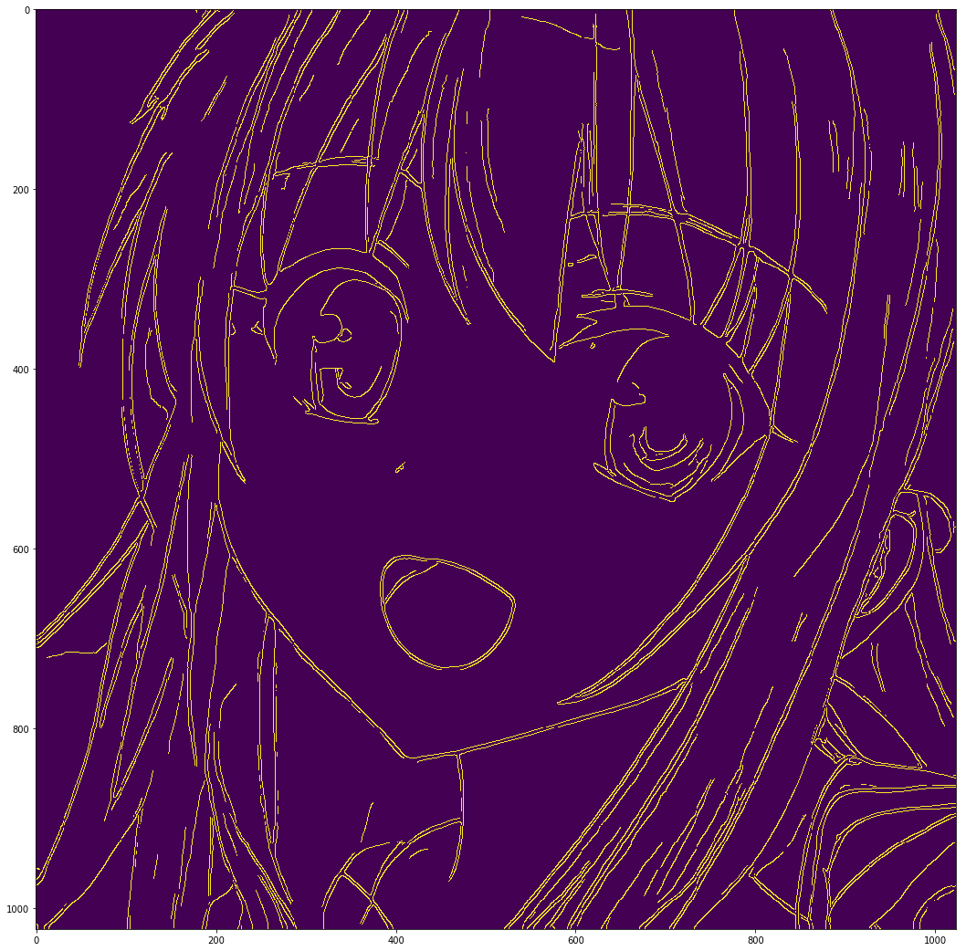
Canny Edge

캐니 엣지 검출기는 1986년 존 캐니(John F. Canny)가 제안한 알고리즘으로, 4단계의 알고리즘을 적용해 잡음에 강한 엣지 검출기입니다. 작동 순서는 아래와 같습니다.

• 캐니 알고리즘의 작동 순서
  1. 노이즈 제거(Noise Reduction) : 5 X 5 가우시안 블러링 필터로 노이즈 제거
  2. 엣지 그래디언트 방향 계산 : Sobel Mask를 사용해 엣지 및 그래디언트 방향 검출
  3. 비최대치 억제(Non-Maximum Suppression) : 그래디언트 방향에서 검출된 엣지 중 가장 큰 값만 선택하고 나머지는 제거.
  4. 이력 스레숄딩(Hysteresis Thresholding) : 두 개의 경계값(Max, Min)을 지정한 후 경계 영역에 있는 픽셀들 중 큰 경계값(Max) 밖의 픽셀과 연결성이 없는 픽셀을 제거.

OpenCV는 위 알고리즘을 구현한 cv2.Canny() 함수를 제공하고 있습니다.

• edges = cv2.Canny(img, threshold1, threshold2[, edges, apertureSize, L2gradient])
  • img : 입력 이미지(Numpy array)
  • threshold1, threshold2 : Hysteresis Thresholding에 사용할 최소, 최대값
  • apertureSize : Sobel Mask에 사용할 커널 크기
  • L2gradient : 그래디언트 강도를 구할 방식을 지정하는 플래그
    • True : L2 Norm 사용
    • False : L1 Norm 사용
  • edges : 엣지 결과값을 리턴받을 2차원 배열

plt.figure(figsize=(60, 20))
left = 0.125
right = 0.7
bottom = 0.2
top = 0.9
wspace = 0.02
hspace = 0.0
plt.subplots_adjust(left=left, right=right, bottom=bottom, top=top, wspace=wspace, hspace=hspace)

# Using Canny API in OpenCV
edges = cv2.Canny(img, 100, 200)

# Print results
plt.imshow(edges)

Fourier transform 응용

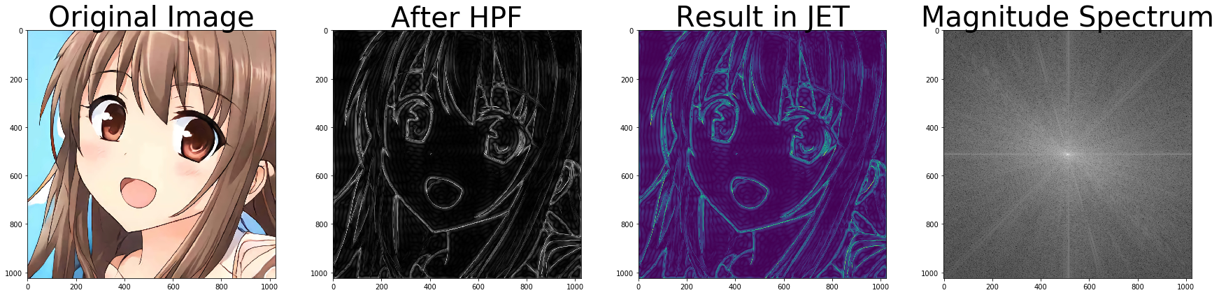
푸리에 트랜스폼은 이미지를 주파수 영역으로 변환한 후 이미지 프로세싱 작업을 수행할 수 있게 해 주며, 주파수 영역에서의 작업이 끝난 후 Inversion Fourier Transform(IFT) 연산을 통해 원래 이미지 영역으로 되돌려 이미지 프로세싱 결과를 확인해 볼 수 있습니다.
이미지는 X, Y 두 방향으로 샘플링되는 이산 신호로 간주할 수 있으며, 이는 즉 푸리에 변환을 X, Y축 두 방향에 대해 수행하면 이미지의 주파수 표현을 얻을 수 있음을 의미합니다.

사인(sin) 곡선의 경우 짧은 시간에 진폭이 빠르게 변화하면 고주파 신호라고 볼 수 있으며, 천천히 변화하면 저주파 신호로 볼 수 있습니다. 따라서 이미지의 edge(가장자리)와 노이즈는 이미지의 고주파 부분이라고 할 수 있으며, 진폭에 큰 변화가 없으면 저주파 성분으로 볼 수 있습니다.

# Original code from https://blog.naver.com/samsjang/220568857153
import numpy as np
import cv2
import matplotlib.pyplot as plt

def Fourier(image):
    image = cv2.cvtColor(image, cv2.COLOR_BGR2GRAY)
    
    f = np.fft.fft2(image)
    fshift = np.fft.fftshift(f)
    magnitude_spectrum = 20*np.log(np.abs(fshift))
    
    rows, cols = image.shape
    print(rows, cols)
    crow, ccol = int(rows/2), int(cols/2)
    
    fshift[crow-30:crow+30, ccol-30:ccol+30]=0
    f_ishift = np.fft.ifftshift(fshift)
    img_back = np.fft.ifft2(f_ishift)
    img_back = np.abs(img_back)
    
    plt.figure(figsize=(30, 30))
    plt.subplot(441)
    plt.imshow(img, cmap='gray')
    plt.title('Original Image', fontsize=40)
    
    plt.subplot(442)
    plt.imshow(img_back, cmap='gray')
    plt.title('After HPF', fontsize=40)
    
    plt.subplot(443)
    plt.imshow(img_back)
    plt.title('Result in JET', fontsize=40)
    
    plt.subplot(444)
    plt.imshow(magnitude_spectrum, cmap = 'gray')
    plt.title('Magnitude Spectrum', fontsize=40)
    
    plt.show() 
    

Fourier(img)

1024 1024