CBIS-DDSM 데이터셋 Simple EDA (上)

10 Dec 2019 in Devlog / Shoveling on Dataset review, Eda

CBIS-DDSM은 유방암 Classfication 또는 Detection 분야에서 종종 사용되는 데이터셋입니다. 이번 포스트에서는 개인 연구에 활용하기 위해 개인적으로 EDA를 수행한 노트북을 다룹니다.

CBIS-DDSM은 유방암 Classfication 또는 Detection 분야에서 종종 사용되는 데이터셋입니다. 이번 포스트에서는 개인 연구에 활용하기 위해 개인적으로 EDA를 수행한 노트북을 다룹니다. 보다 상세한 통계 정보를 다루는 하(下)편은 언제가 될 지는 모르겠으나 빠른 시일 내로 업데이트해 보겠습니다.

CBIS-DDSM_EDA

CBIS-DDSM 데이터셋에서 제공되는 부가 파일들을 활용해 EDA를 수행해 봅니다. CBIS-DDSM 데이터셋은 이미지 데이터(.dcm)와 메타 데이터(.csv)로 구성되며, 이미지 데이터는 아래와 같은 내역으로 구성되어 있습니다.

Dataset format
- Modality : MG(Mammography
- Number of Patients : 6671
- Number of Studies : 6775
- Number of Series : 6775
- Number of Images : 10239
- Entire image size : 163.6GB

전체 이미지는 6671장으로 구성되어 있으며 각 case별 상세 설명이 기재된 네 개의 .csv파일이 제공됩니다. Abnormality type은 ‘Calculation case’와 ‘Mass case’로 나뉘며, Calculation case는 흰색 반점(spots)이나 얼룩덜룩한 형태(flecks)로 관찰되는 Abnormality type을 의미하고, Mass case는 Breast Lumps가 구름처럼 mass하게 퍼져 있는 Abnormality type을 의미합니다.

calc_case_description_train_set.csv: 두 개의 abnormality type 중 calc(calcification, 석회화 조직)인 case들을 모아 구성된 train set list입니다.
calc_case_description_test_set.csv: 두 개의 abnormality type 중 calc인 case들을 모아 구성된 test set list입니다.
mass_case_description_train_set.csv: 두 개의 abnormality type 중 mass(mass lumps, 덩어리 조직)인 case들을 모아 구성된 train set list입니다.
mass_case_description_test_set.csv: 두 개의 abnormality type 중 mass인 case들을 모아 구성된 test set list입니다.

EDA에 앞서, 데이터셋을 한바퀴 둘러보겠습니다.

1. 데이터셋 둘러보기

1.1 `Abnormality type`별 feature 탐색

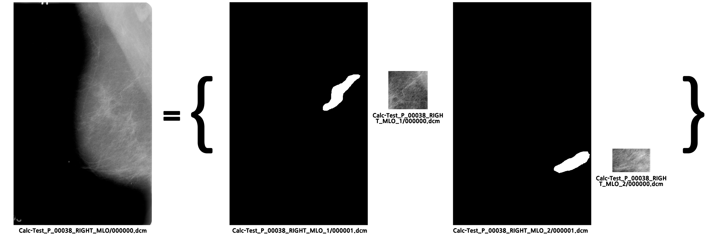
Abnormality type의 구분은 파일명에서 calc와 mass 접두사로 되어 있습니다. 각 사례(case)는 ①원본 이미지와, ②원본 이미지에 대응되는 segment annotation과, 해당 segment annotation을 포함하는 ③bounding box를 crop한 이미지를 포함하고 있습니다. 이 꼭지에서는 Abnormality type별 각 컬럼의 feature가 의미하는 바를 알아 보도록 하겠습니다.

case_details

import os
import pandas as pd

# Setting base path
ROOT_PATH = os.path.join(os.getcwd(), 'Dataset_csv')
CBISDDSM_csvPATH = os.path.join(ROOT_PATH, 'CBISDDSM')
MIAS_PATH = os.path.join(ROOT_PATH, 'MIAS')

# Load Dataframe from .csv
calc_case_description_train_set_df = pd.read_csv(os.path.join(CBISDDSM_csvPATH, "calc_case_description_train_set.csv"), index_col=0)
calc_case_description_test_set_df = pd.read_csv(os.path.join(CBISDDSM_csvPATH, "calc_case_description_test_set.csv"), index_col=0)
mass_case_description_train_set_df = pd.read_csv(os.path.join(CBISDDSM_csvPATH, "mass_case_description_train_set.csv"), index_col=0)
mass_case_description_test_set_df = pd.read_csv(os.path.join(CBISDDSM_csvPATH, "mass_case_description_test_set.csv"), index_col=0)

# 몇 가지 테스트 및 데이터 타입 조사를 위한 더미 코드입니다.
# print(calc_case_description_train_set_df['abnormality type'].unique())
# print(calc_case_description_test_set_df['abnormality type'].unique())
print(mass_case_description_train_set_df['subtlety'].unique())
print(mass_case_description_train_set_df['abnormality id']['P_00001'])
print(mass_case_description_test_set_df['subtlety'].unique())

[4 3 5 1 2 0]
P_00001    1
P_00001    1
Name: abnormality id, dtype: int64
[5 4 2 3 1]

각 .csv파일은 아래와 같은 내용들을 포함하고 있습니다. 각 column에 대한 설명은 다음과 같으며, 보다 자세한 설명은 https://www.nature.com/articles/sdata2017177에서 확인하실 수 있습니다. (중복 feature가 존재하는 경우는 dataframe['columnname'].unique()로 유니크한 값만 뽑아 확인)

calcification 타입의 데이터셋 각 컬럼별 설명 (calc_case_description_train_set_df, calc_case_description_test_set_df)
- patient_id: 신원 정보가 제거된(de-identification) 환자 번호입니다. (e.g. P_00005, P_00013, …)
- breast density: 유방 조직의 밀도를 구분한 정수형 feature입니다. train csv에는 1에서 4까지의 int형 feature를, test csv에는 0~4의 int형 feature를 포함하고 있습니다. (e.g. 3, 4, 1, 2, …)
- left or right breast: 유방을 촬영한 각도입니다. LEFT, RIGHT로 구성된 srt형 바이너리 feature입니다. (e.g. LEFT, RIGHT, …)
- image view: mammography 촬영 방법에 따른 구분입니다. CC, MLO로 구성된 str형 바이너리 feature입니다. (e.g. CC, MLO, …)
- abnormality id: 해당 case 안에 anomaly 패치가 몇 개인지 구분하기 위한 id입니다. train csv는 1부터 7까지의 범위를 갖는 int형 feature를, test csv는 1~5의 범위를 갖는 int형 feature를 포함하고 있습니다. (e.g. 3, 2, 5, 1, …)
- abnormality type: Abnormality type에 따른 구분입니다. train과 test로 나뉜 네 개의 .csv파일에서 해당 테이블은 파일에 대해 모두 동일한 값을 가지며, calcification과 mass 두 타입이 존재합니다. 아래 dataframe.head를 통해 해당 column 정보를 확인하실 수 있습니다.
- calc type: calcification 타입의 lumps(덩어리)에서 나타나는 Cancer diagnostic 정보입니다. 46종으로 구분되어 있으며, str형 feature입니다. (e.g. AMORPHOUS, ROUND_AND_REGULAR-AMORPHOUS, …)
- calc distribution: calc타입의 lumps 조직이 얼마나 뭉쳐 있는지, 퍼져 있는지에 대한 str형 feature입니다. CLUSTERED, LINEAR, REGIONAL, DIFFUSELY_SCATTERED, SEGMENTAL, CLUSTERED-LINEAR, CLUSTERED-SEGMENTAL, LINEAR-SEGMENTAL, REGIONAL-REGIONAL로 구성되어 있으며, nan값도 포함되어 있으므로 핸들링에 주의가 필요합니다. (e.g. CLUSTERED-LINEAR, SEGMENTAL, CLUSTERED, …)
- assessment: 비정상 정도에 대한 레벨을 구분하는 정수형 feature입니다. BI-RADS에 따른 각 사례별 분류로, 0, 2, 3, 4, 5의 unique한 int형 features가 포함되어 있습니다.
- pathology: 해당 lumps에 대한 병리학적 분류를 의미합니다. BENIGN_WITHOUT_CALLBACK, BENIGN, MALIGNANT 세 개의 unique한 str형 features로 구성되어 있으며, 각각 정상(추정), 양성, 음성을 의미합니다. (e.g. BENIGN, BENIGN, MALIGNANT, …)
- subtlety: 확인되지 않은 컬럼입니다. 1~5의 범위를 갖는 int형 feature로 구성되어 있습니다. (e.g. 3, 4, 1, 5, 2, …)
- image file path: 원본 이미지 파일(.dcm)의 경로입니다.
- cropped image file path: 의심 ROI segment에 대해 crop 후 저장한 .dcm 이미지 경로입니다. segment 단위로 bounding box를 근사해 crop한 것으로 추정됩니다.
- ROI mask file path: 원본 이미지 파일에 대응해 의심 ROI 영역을 segment로 annotation한 마스크 .dcm 이미지입니다.
mass 타입의 데이터셋 각 컬럼별 설명 (mass_case_description_train_set_df, mass_case_description_test_set_df)
- patient_id: 상기와 동일
- breast density: 유방 조직의 밀도를 구분한 정수형 feature입니다. train csv와 test csv 모두 1~4의 int형 feature를 포함하고 있습니다. (e.g. 3, 4, 1, 2, …)
- left or right breast: 상기와 동일
- image view: 상기와 동일
- abnormality id: 비정상 정도에 대한 레벨을 구분하는 정수형 feature입니다. BI-RADS에 따른 각 사례별 분류로 추정되며, train csv는 1부터 6까지의 범위를 갖는 int형 feature를, test csv는 1~4의 범위를 갖는 int형 feature를 포함하고 있습니다. (e.g. 3, 2, 5, 1, …)
- abnormality type: 상기와 동일
- mass shape: mass 타입의 lumps 조직이 어떤 모양을 갖고 있는지에 대한 정보입니다. 약 19개의 str형 features로 구분되어 있습니다. nan값도 포함되어 있으므로 핸들링에 주의가 필요합니다. (e.g. IRREGULAR-ARCHITECTURAL_DISTORTION, LOBULATED, …)
- mass margins: 확인되지 않은 컬럼입니다. SPICULATED, ILL_DEFINED, CIRCUMSCRIBED, ILL_DEFINED-SPICULATED, OBSCURED, OBSCURED-ILL_DEFINED, MICROLOBULATED, MICROLOBULATED-ILL_DEFINED-SPICULATED, MICROLOBULATED-SPICULATED, CIRCUMSCRIBED-ILL_DEFINED, MICROLOBULATED-ILL_DEFINED, CIRCUMSCRIBED-OBSCURED, OBSCURED-SPICULATED, OBSCURED-ILL_DEFINED-SPICULATED, CIRCUMSCRIBED-MICROLOBULATED의 unique한 str features를 갖고 있으며 nan값도 포함되어 있으므로 핸들링에 주의가 필요합니다. (e.g. CIRCUMSCRIBED, SPICULATED, …)
- assessment: 확인되지 않은 컬럼입니다. 0~5의 unique한 int형 features가 포함되어 있습니다.
- pathology: 상기와 동일
- subtlety: 확인되지 않은 컬럼입니다. train csv는 1부터 5까지의 범위를 갖는 int형 feature로 구성되어 있으며, test csv는 1~5의 범위를 갖는 int형 features로 구성되어 있습니다. (e.g. 3, 4, 1, 5, 2, …)
- image file path, cropped image file path, ROI mask file path: 상기와 동일

calc_case_description_train_set_df.head(3)

	breast density	left or right breast	image view	abnormality id	abnormality type	calc type	calc distribution	assessment	pathology	subtlety	image file path	cropped image file path	ROI mask file path
patient_id
P_00005	3	RIGHT	CC	1	calcification	AMORPHOUS	CLUSTERED	3	MALIGNANT	3	Calc-Training_P_00005_RIGHT_CC/1.3.6.1.4.1.959...	Calc-Training_P_00005_RIGHT_CC_1/1.3.6.1.4.1.9...	Calc-Training_P_00005_RIGHT_CC_1/1.3.6.1.4.1.9...
P_00005	3	RIGHT	MLO	1	calcification	AMORPHOUS	CLUSTERED	3	MALIGNANT	3	Calc-Training_P_00005_RIGHT_MLO/1.3.6.1.4.1.95...	Calc-Training_P_00005_RIGHT_MLO_1/1.3.6.1.4.1....	Calc-Training_P_00005_RIGHT_MLO_1/1.3.6.1.4.1....
P_00007	4	LEFT	CC	1	calcification	PLEOMORPHIC	LINEAR	4	BENIGN	4	Calc-Training_P_00007_LEFT_CC/1.3.6.1.4.1.9590...	Calc-Training_P_00007_LEFT_CC_1/1.3.6.1.4.1.95...	Calc-Training_P_00007_LEFT_CC_1/1.3.6.1.4.1.95...

calc_case_description_test_set_df.head(3)

	breast density	left or right breast	image view	abnormality id	abnormality type	calc type	calc distribution	assessment	pathology	subtlety	image file path	cropped image file path	ROI mask file path
patient_id
P_00038	2	LEFT	CC	1	calcification	PUNCTATE-PLEOMORPHIC	CLUSTERED	4	BENIGN	2	Calc-Test_P_00038_LEFT_CC/1.3.6.1.4.1.9590.100...	Calc-Test_P_00038_LEFT_CC_1/1.3.6.1.4.1.9590.1...	Calc-Test_P_00038_LEFT_CC_1/1.3.6.1.4.1.9590.1...
P_00038	2	LEFT	MLO	1	calcification	PUNCTATE-PLEOMORPHIC	CLUSTERED	4	BENIGN	2	Calc-Test_P_00038_LEFT_MLO/1.3.6.1.4.1.9590.10...	Calc-Test_P_00038_LEFT_MLO_1/1.3.6.1.4.1.9590....	Calc-Test_P_00038_LEFT_MLO_1/1.3.6.1.4.1.9590....
P_00038	2	RIGHT	CC	1	calcification	VASCULAR	NaN	2	BENIGN_WITHOUT_CALLBACK	5	Calc-Test_P_00038_RIGHT_CC/1.3.6.1.4.1.9590.10...	Calc-Test_P_00038_RIGHT_CC_1/1.3.6.1.4.1.9590....	Calc-Test_P_00038_RIGHT_CC_1/1.3.6.1.4.1.9590....

mass_case_description_train_set_df.head(3)

	breast_density	left or right breast	image view	abnormality id	abnormality type	mass shape	mass margins	assessment	pathology	subtlety	image file path	cropped image file path	ROI mask file path
patient_id
P_00001	3	LEFT	CC	1	mass	IRREGULAR-ARCHITECTURAL_DISTORTION	SPICULATED	4	MALIGNANT	4	Mass-Training_P_00001_LEFT_CC/1.3.6.1.4.1.9590...	Mass-Training_P_00001_LEFT_CC_1/1.3.6.1.4.1.95...	Mass-Training_P_00001_LEFT_CC_1/1.3.6.1.4.1.95...
P_00001	3	LEFT	MLO	1	mass	IRREGULAR-ARCHITECTURAL_DISTORTION	SPICULATED	4	MALIGNANT	4	Mass-Training_P_00001_LEFT_MLO/1.3.6.1.4.1.959...	Mass-Training_P_00001_LEFT_MLO_1/1.3.6.1.4.1.9...	Mass-Training_P_00001_LEFT_MLO_1/1.3.6.1.4.1.9...
P_00004	3	LEFT	CC	1	mass	ARCHITECTURAL_DISTORTION	ILL_DEFINED	4	BENIGN	3	Mass-Training_P_00004_LEFT_CC/1.3.6.1.4.1.9590...	Mass-Training_P_00004_LEFT_CC_1/1.3.6.1.4.1.95...	Mass-Training_P_00004_LEFT_CC_1/1.3.6.1.4.1.95...

mass_case_description_test_set_df.head(3)

	breast_density	left or right breast	image view	abnormality id	abnormality type	mass shape	mass margins	assessment	pathology	subtlety	image file path	cropped image file path	ROI mask file path
patient_id
P_00016	4	LEFT	CC	1	mass	IRREGULAR	SPICULATED	5	MALIGNANT	5	Mass-Test_P_00016_LEFT_CC/1.3.6.1.4.1.9590.100...	Mass-Test_P_00016_LEFT_CC_1/1.3.6.1.4.1.9590.1...	Mass-Test_P_00016_LEFT_CC_1/1.3.6.1.4.1.9590.1...
P_00016	4	LEFT	MLO	1	mass	IRREGULAR	SPICULATED	5	MALIGNANT	5	Mass-Test_P_00016_LEFT_MLO/1.3.6.1.4.1.9590.10...	Mass-Test_P_00016_LEFT_MLO_1/1.3.6.1.4.1.9590....	Mass-Test_P_00016_LEFT_MLO_1/1.3.6.1.4.1.9590....
P_00017	2	LEFT	CC	1	mass	ROUND	CIRCUMSCRIBED	4	MALIGNANT	4	Mass-Test_P_00017_LEFT_CC/1.3.6.1.4.1.9590.100...	Mass-Test_P_00017_LEFT_CC_1/1.3.6.1.4.1.9590.1...	Mass-Test_P_00017_LEFT_CC_1/1.3.6.1.4.1.9590.1...

print('Length of calc_case_description_train_set_df: ', len(calc_case_description_train_set_df))
print('Length of calc_case_description_test_set_df', len(calc_case_description_test_set_df))
print('Length of mass_case_description_train_set_df: ', len(mass_case_description_train_set_df))
print('Length of mass_case_description_test_set_df:', len(mass_case_description_test_set_df))

Length of calc_case_description_train_set_df:  1546
Length of calc_case_description_test_set_df 326
Length of mass_case_description_train_set_df:  1318
Length of mass_case_description_test_set_df: 378

1.2 `Abnormality type`별 이미지 관찰

이제 calc와 mass 두 가지 타입 별로 이미지 몇 장을 뽑아 시각화해 보겠습니다. 각 column의 인덱스는 다음과 같이 patient_id로 접근할 수 있습니다. 우선 3개 정도의 이미지를 랜덤 샘플링해 출력해 보겠습니다.

sample_calc_case_description_train_set_df = calc_case_description_train_set_df.sample(n=3)
sample_mass_case_description_train_set_df = mass_case_description_train_set_df.sample(n=3)

sample_calc_case_description_train_set_df

	breast density	left or right breast	image view	abnormality id	abnormality type	calc type	calc distribution	assessment	pathology	subtlety	image file path	cropped image file path	ROI mask file path
patient_id
P_01830	3	RIGHT	MLO	3	calcification	PUNCTATE	REGIONAL	2	BENIGN_WITHOUT_CALLBACK	5	Calc-Training_P_01830_RIGHT_MLO/1.3.6.1.4.1.95...	Calc-Training_P_01830_RIGHT_MLO_3/1.3.6.1.4.1....	Calc-Training_P_01830_RIGHT_MLO_3/1.3.6.1.4.1....
P_01002	3	LEFT	CC	1	calcification	FINE_LINEAR_BRANCHING	REGIONAL	5	MALIGNANT	5	Calc-Training_P_01002_LEFT_CC/1.3.6.1.4.1.9590...	Calc-Training_P_01002_LEFT_CC_1/1.3.6.1.4.1.95...	Calc-Training_P_01002_LEFT_CC_1/1.3.6.1.4.1.95...
P_01136	2	RIGHT	MLO	1	calcification	PLEOMORPHIC	CLUSTERED	5	MALIGNANT	5	Calc-Training_P_01136_RIGHT_MLO/1.3.6.1.4.1.95...	Calc-Training_P_01136_RIGHT_MLO_1/1.3.6.1.4.1....	Calc-Training_P_01136_RIGHT_MLO_1/1.3.6.1.4.1....

sample_mass_case_description_train_set_df

	breast_density	left or right breast	image view	abnormality id	abnormality type	mass shape	mass margins	assessment	pathology	subtlety	image file path	cropped image file path	ROI mask file path
patient_id
P_00528	3	LEFT	MLO	2	mass	OVAL	CIRCUMSCRIBED	3	BENIGN	5	Mass-Training_P_00528_LEFT_MLO/1.3.6.1.4.1.959...	Mass-Training_P_00528_LEFT_MLO_2/1.3.6.1.4.1.9...	Mass-Training_P_00528_LEFT_MLO_2/1.3.6.1.4.1.9...
P_01163	2	LEFT	CC	1	mass	OVAL	SPICULATED	4	MALIGNANT	5	Mass-Training_P_01163_LEFT_CC/1.3.6.1.4.1.9590...	Mass-Training_P_01163_LEFT_CC_1/1.3.6.1.4.1.95...	Mass-Training_P_01163_LEFT_CC_1/1.3.6.1.4.1.95...
P_00847	4	LEFT	MLO	1	mass	ARCHITECTURAL_DISTORTION	NaN	2	BENIGN	4	Mass-Training_P_00847_LEFT_MLO/1.3.6.1.4.1.959...	Mass-Training_P_00847_LEFT_MLO_1/1.3.6.1.4.1.9...	Mass-Training_P_00847_LEFT_MLO_1/1.3.6.1.4.1.9...

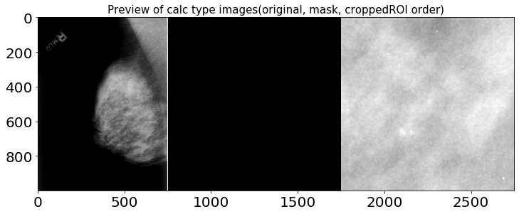
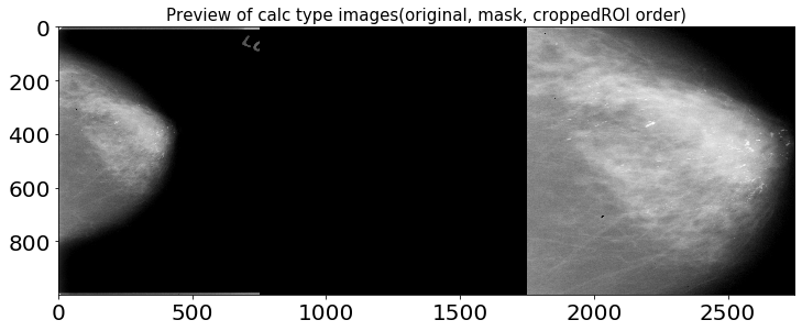
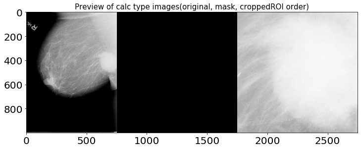
1.2.1. `calc` 타입 이미지 확인

샘플 오리지널 이미지와 cropped ROI, ROI mask의 이미지 비율은 각각 다르지만 시각화의 편의를 위해 1000 x 1000 해상도로 출력했습니다.

import PIL
import numpy as np
import pydicom as dicom
from PIL import ImageDraw
import matplotlib.pyplot as plt
import cv2

font = cv2.FONT_HERSHEY_SIMPLEX
fontScale = 0.5

# Dataset directory
DDSM_dataPATH = 'E:/CBIM-DDSM'

# sample image file lists
calc_case_original_img = sample_calc_case_description_train_set_df['image file path'].to_list()
calc_case_croppedROI_img = sample_calc_case_description_train_set_df['cropped image file path'].to_list()
calc_case_ROImask_img = sample_calc_case_description_train_set_df['ROI mask file path'].to_list()

for i in range(3):
    plt.figure(figsize=(12,20))
    original_image_ds = dicom.dcmread(os.path.join(DDSM_dataPATH, calc_case_original_img[i]).replace('\n', '').replace('\r', ''))
    original_image_ds_resized = cv2.resize(original_image_ds.pixel_array, dsize=(750, 1000), interpolation=cv2.INTER_CUBIC)

    croppedROI_image_ds = dicom.dcmread(os.path.join(DDSM_dataPATH, calc_case_croppedROI_img[i]).replace('\n', '').replace('\r', ''))
    croppedROI_image_ds_resized = cv2.resize(croppedROI_image_ds.pixel_array, dsize=(1000, 1000), interpolation=cv2.INTER_CUBIC)

    ROIMask_image_ds = dicom.dcmread(os.path.join(DDSM_dataPATH, calc_case_ROImask_img[i]).replace('\n', '').replace('\r', ''))
    ROIMask_image_ds_resized = cv2.resize(ROIMask_image_ds.pixel_array, dsize=(1000, 1000), interpolation=cv2.INTER_CUBIC)
    merged_image = np.concatenate((np.concatenate((original_image_ds_resized, croppedROI_image_ds_resized), axis=1), ROIMask_image_ds_resized), axis=1)
        
    plt.title('Preview of calc type images(original, mask, croppedROI order)', fontsize=15)
    plt.imshow(merged_image, cmap = 'gray')
    plt.show()

case_details

1.2.2. `mass` 타입 이미지 확인

font = cv2.FONT_HERSHEY_SIMPLEX
fontScale = 0.5

# sample image file lists
mass_case_original_img = sample_mass_case_description_train_set_df['image file path'].to_list()
mass_case_croppedROI_img = sample_mass_case_description_train_set_df['cropped image file path'].to_list()
mass_case_ROImask_img = sample_mass_case_description_train_set_df['ROI mask file path'].to_list()

for i in range(3):
    plt.figure(figsize=(12,20))
    original_image_ds = dicom.dcmread(os.path.join(DDSM_dataPATH, mass_case_original_img[i].replace('\n', '').replace('\r', '')))
    original_image_ds_resized = cv2.resize(original_image_ds.pixel_array, dsize=(750, 1000), interpolation=cv2.INTER_CUBIC)

    croppedROI_image_ds = dicom.dcmread(os.path.join(DDSM_dataPATH, mass_case_croppedROI_img[i].replace('\n', '').replace('\r', '')))
    croppedROI_image_ds_resized = cv2.resize(croppedROI_image_ds.pixel_array, dsize=(1000, 1000), interpolation=cv2.INTER_CUBIC)

    ROIMask_image_ds = dicom.dcmread(os.path.join(DDSM_dataPATH, mass_case_ROImask_img[i].replace('\n', '').replace('\r', '')))
    ROIMask_image_ds_resized = cv2.resize(ROIMask_image_ds.pixel_array, dsize=(1000, 1000), interpolation=cv2.INTER_CUBIC)
    merged_image = np.concatenate((np.concatenate((original_image_ds_resized, croppedROI_image_ds_resized), axis=1), ROIMask_image_ds_resized), axis=1)
        
    plt.title('Preview of mass type images', fontsize=15)
    plt.imshow(merged_image, cmap = 'gray')
    plt.show()

case_details

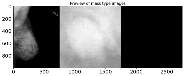
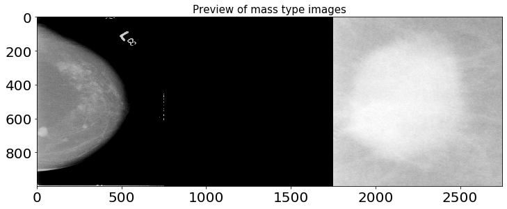
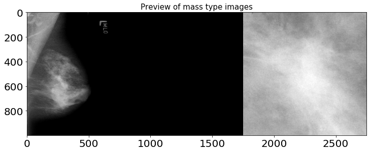
위 이미지들을 통해 확인할 수 있듯, cropped ROI에는 히스토그램 평활화로 추정되는 이미지 전처리 기법이 적용되어 있습니다. X-Ray 이미지를 전처리하는 데엔 다양한 방법들이 존재하며, 아래 노트북을 참고해 전처리 및 Augmentaion 작업을 진행하면 큰 도움이 될 것으로 예상됩니다.

https://github.com/yuyuyu123456/CBIS-DDSM/blob/master/EDA.ipynb

2. CSV data EDA

이제 각 csv 파일이 갖고 있는 column들에 대해 보다 자세히 EDA를 수행한 후 분포를 확인해 보도록 하겠습니다. 각 csv파일들이 갖고 있는 정수형 변수들에 대한 간단한 통계 정보는 아래와 같습니다.

calc_case_description_train_set_df.describe()

	breast density	abnormality id	assessment	subtlety
count	1546.000000	1546.000000	1546.000000	1546.000000
mean	2.663648	1.415265	3.258732	3.411384
std	0.937219	0.903571	1.229231	1.179754
min	1.000000	1.000000	0.000000	1.000000
25%	2.000000	1.000000	2.000000	3.000000
50%	3.000000	1.000000	4.000000	3.000000
75%	3.000000	1.000000	4.000000	4.000000
max	4.000000	7.000000	5.000000	5.000000

calc_case_description_test_set_df.describe()

	breast density	abnormality id	assessment	subtlety
count	326.000000	326.000000	326.000000	326.000000
mean	2.696319	1.214724	3.453988	3.319018
std	0.909667	0.529061	1.188159	1.188175
min	0.000000	1.000000	0.000000	1.000000
25%	2.000000	1.000000	2.000000	3.000000
50%	3.000000	1.000000	4.000000	3.000000
75%	3.000000	1.000000	4.000000	4.000000
max	4.000000	5.000000	5.000000	5.000000

mass_case_description_train_set_df.describe()

	breast_density	abnormality id	assessment	subtlety
count	1318.000000	1318.000000	1318.000000	1318.000000
mean	2.203338	1.116085	3.504552	3.965857
std	0.873774	0.467013	1.414609	1.102032
min	1.000000	1.000000	0.000000	0.000000
25%	2.000000	1.000000	3.000000	3.000000
50%	2.000000	1.000000	4.000000	4.000000
75%	3.000000	1.000000	4.000000	5.000000
max	4.000000	6.000000	5.000000	5.000000

mass_case_description_test_set_df.describe()

	breast_density	abnormality id	assessment	subtlety
count	378.000000	378.000000	378.000000	378.000000
mean	2.396825	1.092593	3.534392	3.785714
std	0.859455	0.398136	1.343076	1.171776
min	1.000000	1.000000	0.000000	1.000000
25%	2.000000	1.000000	3.000000	3.000000
50%	2.000000	1.000000	4.000000	4.000000
75%	3.000000	1.000000	4.000000	5.000000
max	4.000000	4.000000	5.000000	5.000000

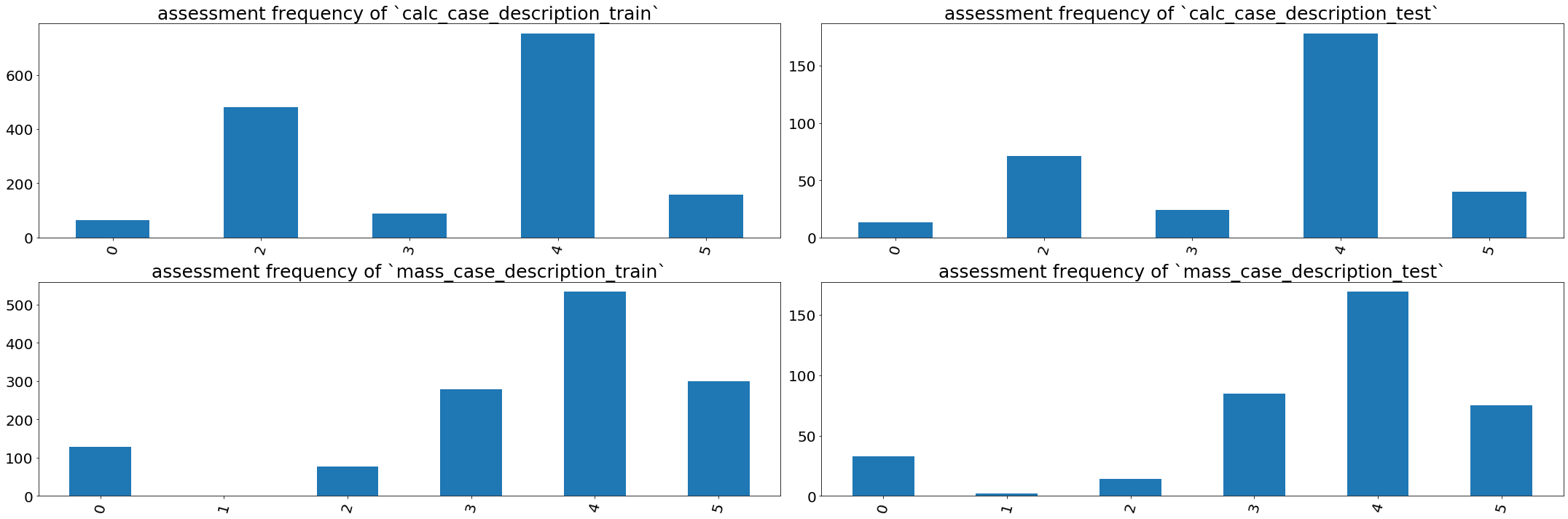
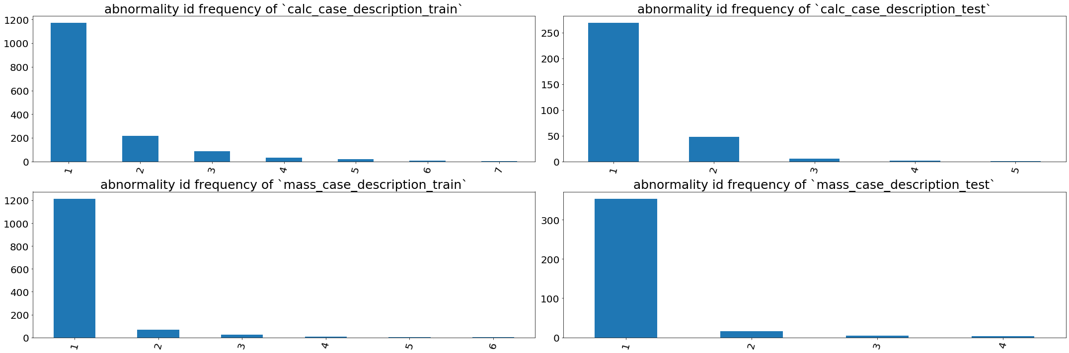
2.1 `assessment` and `abnormality id` distribution

우선, assessment와 abnormality id의 분포를 출력해 보겠습니다. assessment는 목적을 확인할 수 없는 컬럼이고, abnormality id는 BI-RADS 기준에 따라 분류된 비정상 정도를 의미합니다.

import matplotlib
import matplotlib.pylab as pylab
import matplotlib.pyplot as plt

SMALL_SIZE = 17
MEDIUM_SIZE = 20
BIGGER_SIZE = 25
font = {'family' : 'DejaVu Sans',
        'weight' : 'normal',}
matplotlib.rc('font', **font)
params = {'legend.fontsize': SMALL_SIZE,
         'axes.labelsize': MEDIUM_SIZE,
         'axes.titlesize':BIGGER_SIZE,
         'xtick.labelsize':MEDIUM_SIZE,
         'ytick.labelsize':MEDIUM_SIZE}
pylab.rcParams.update(params)

fig, axes = plt.subplots(nrows=2, ncols=2)

calc_case_description_train_set_df['assessment'].value_counts().sort_index().plot(ax=axes[0, 0], kind='bar', rot=75, figsize=(20, 10)).set_title('assessment frequency of `calc_case_description_train`')
calc_case_description_test_set_df['assessment'].value_counts().sort_index().plot(ax=axes[0, 1], kind='bar', rot=75, figsize=(20, 10)).set_title('assessment frequency of `calc_case_description_test`')
mass_case_description_train_set_df['assessment'].value_counts().sort_index().plot(ax=axes[1, 0], kind='bar', rot=75, figsize=(30, 10)).set_title('assessment frequency of `mass_case_description_train`')
mass_case_description_test_set_df['assessment'].value_counts().sort_index().plot(ax=axes[1, 1], kind='bar', rot=75, figsize=(30, 10)).set_title('assessment frequency of `mass_case_description_test`')

plt.tight_layout()
plt.show()

case_details

import matplotlib
import matplotlib.pylab as pylab
import matplotlib.pyplot as plt

SMALL_SIZE = 17
MEDIUM_SIZE = 20
BIGGER_SIZE = 25
font = {'family' : 'DejaVu Sans',
        'weight' : 'normal',}
matplotlib.rc('font', **font)
params = {'legend.fontsize': SMALL_SIZE,
         'axes.labelsize': MEDIUM_SIZE,
         'axes.titlesize':BIGGER_SIZE,
         'xtick.labelsize':MEDIUM_SIZE,
         'ytick.labelsize':MEDIUM_SIZE}
pylab.rcParams.update(params)

fig, axes = plt.subplots(nrows=2, ncols=2)

calc_case_description_train_set_df['abnormality id'].value_counts().sort_index().plot(ax=axes[0, 0], kind='bar', rot=75, figsize=(20, 10)).set_title('abnormality id frequency of `calc_case_description_train`')
calc_case_description_test_set_df['abnormality id'].value_counts().sort_index().plot(ax=axes[0, 1], kind='bar', rot=75, figsize=(20, 10)).set_title('abnormality id frequency of `calc_case_description_test`')
mass_case_description_train_set_df['abnormality id'].value_counts().sort_index().plot(ax=axes[1, 0], kind='bar', rot=75, figsize=(30, 10)).set_title('abnormality id frequency of `mass_case_description_train`')
mass_case_description_test_set_df['abnormality id'].value_counts().sort_index().plot(ax=axes[1, 1], kind='bar', rot=75, figsize=(30, 10)).set_title('abnormality id frequency of `mass_case_description_test`')

plt.tight_layout()
plt.show()

case_details

2.2 Pathology(`normal`, `benign`, `malignant`) distribution

그 다음으로, 학습에 가장 중요한 영향을 끼칠 Pathology column에 대해서도 분포를 출력해 보겠습니다.

import matplotlib
import matplotlib.pylab as pylab
import matplotlib.pyplot as plt

SMALL_SIZE = 17
MEDIUM_SIZE = 20
BIGGER_SIZE = 25
font = {'family' : 'DejaVu Sans',
        'weight' : 'normal',}
matplotlib.rc('font', **font)
params = {'legend.fontsize': SMALL_SIZE,
         'axes.labelsize': MEDIUM_SIZE,
         'axes.titlesize':BIGGER_SIZE,
         'xtick.labelsize':MEDIUM_SIZE,
         'ytick.labelsize':MEDIUM_SIZE}
pylab.rcParams.update(params)

fig, axes = plt.subplots(nrows=2, ncols=2)

calc_case_description_train_set_df['pathology'].value_counts().sort_index().plot(ax=axes[0, 0], kind='bar', rot=0, figsize=(20, 10)).set_title('pathology distribution of `calc_case_description_train`')
calc_case_description_test_set_df['pathology'].value_counts().sort_index().plot(ax=axes[0, 1], kind='bar', rot=0, figsize=(20, 10)).set_title('pathology distribution of `calc_case_description_test`')
mass_case_description_train_set_df['pathology'].value_counts().sort_index().plot(ax=axes[1, 0], kind='bar', rot=0, figsize=(30, 10)).set_title('pathology distribution of `mass_case_description_train`')
mass_case_description_test_set_df['pathology'].value_counts().sort_index().plot(ax=axes[1, 1], kind='bar', rot=0, figsize=(30, 10)).set_title('pathology distribution of `mass_case_description_test`')

plt.tight_layout()
plt.show()

case_details

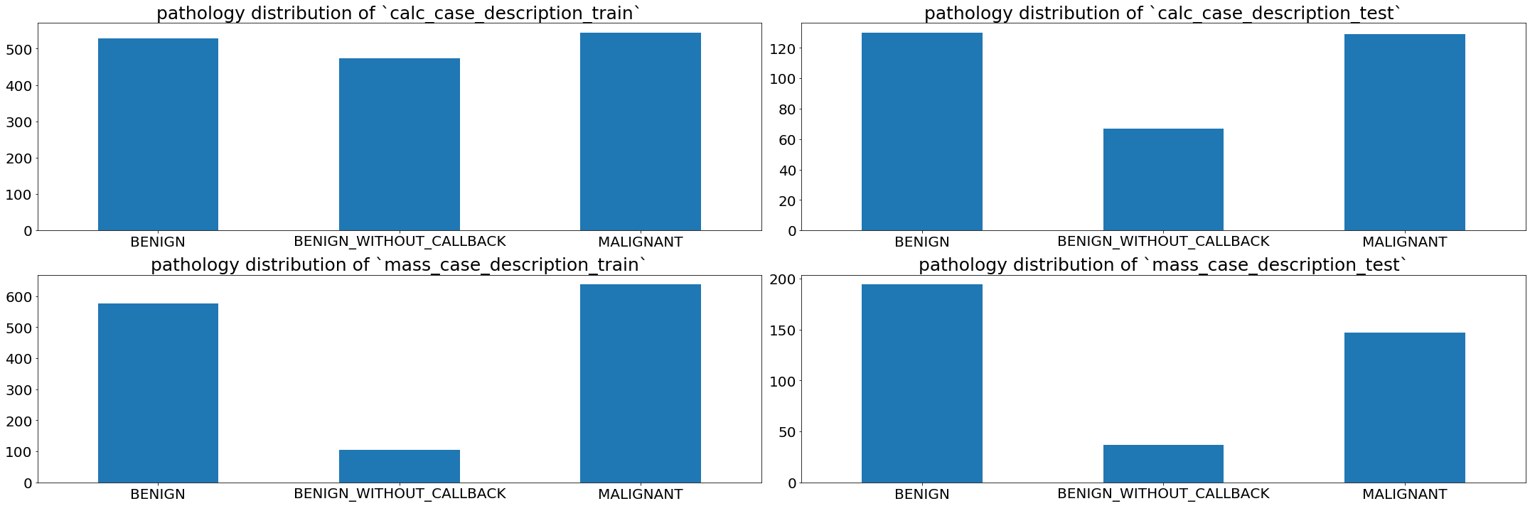
pathology column은 train과 test csv에서 각기 다른 양상을 보이는 것을 확인할 수 있습니다. 이어지는 내용은 下편에서 다루도록 하겠습니다.

CBIS-DDSM 데이터셋 Simple EDA (上)

CBIS-DDSM_EDA

1. 데이터셋 둘러보기

1.1 `Abnormality type`별 feature 탐색

1.2 `Abnormality type`별 이미지 관찰

1.2.1. `calc` 타입 이미지 확인

1.2.2. `mass` 타입 이미지 확인

2. CSV data EDA

2.1 `assessment` and `abnormality id` distribution

2.2 Pathology(`normal`, `benign`, `malignant`) distribution

BrStar Devlog

Error

CBIS-DDSM_EDA

1. 데이터셋 둘러보기

1.1 Abnormality type별 feature 탐색

1.2 Abnormality type별 이미지 관찰

1.2.1. calc 타입 이미지 확인

1.2.2. mass 타입 이미지 확인

2. CSV data EDA

2.1 assessment and abnormality id distribution

2.2 Pathology(normal, benign, malignant) distribution

Templates (for web app):

Error

1.1 `Abnormality type`별 feature 탐색

1.2 `Abnormality type`별 이미지 관찰

1.2.1. `calc` 타입 이미지 확인

1.2.2. `mass` 타입 이미지 확인

2.1 `assessment` and `abnormality id` distribution

2.2 Pathology(`normal`, `benign`, `malignant`) distribution